An overview of Word2Vec

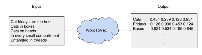
Word2Vec (W2V) is an algorithm that takes in a text corpus and outputs a vector representation for each word, as depicted in the image below:

There are two algorithms that can generate word to vector representations, namely Continuous Bag-of-words and Continuous Skip-gram models.

In the Continuous Bag-of-words model the task of the neural network is to predict a word given the context its context. In the Skip-gram model the task of the neural network is the opposite: to predict the context given the word. 

This post will focus on the Skip-gram model. For more information on the continuous bag of words check out this article.

The literature describes the algorithm in two main ways. The first being as a neural network and the second as a matrix factorisation problem.  This post will follow the neural network based description.

If you are familiar with neural networks already, you can think of Word2Vec as a neural network where the input is a word and the output is a probability of that word forming part of a particular context. The resulting vectors for each word are then the weights leading from  the word’s input node towards the hidden layer.

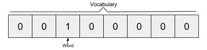
The Skip-gram model takes in a corpus of text and creates a hot-vector for each word. A hot vector is a vector representation of a word where the vector is the size of the vocabulary (total unique words). All dimensions are set to 0 except the dimension representing the word that is used as an input at that point in time. Here is an example of a hot vector:

The above input is given to a neural network with a single hidden layer which looks as follows:

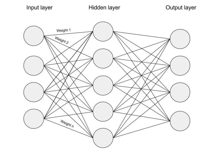
Each dimension of the input passes through each node of the hidden layer. The dimension is multiplied by the weight leading it to the hidden layer. Because the input is a hot vector, only one of the input nodes will have a non-zero value (namely the value of 1). This means that for a particular word only the weights associated with the input node with value 1 will be activated, as shown in the image below:

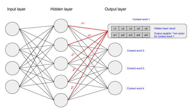
As the input in this case is a hot vector, only one of the input nodes will have a non-zero value. This means that only the weights connected to that input node will be activated in the hidden nodes. An example of the weights that will be taken into account is depicted below for the second word in the vocabulary:

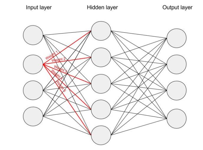
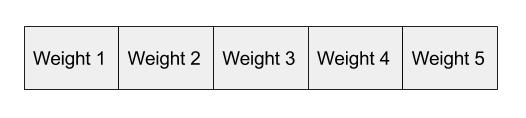
The vector representation of the second word in the vocabulary (shown in the neural network above) will look as follows, once activated in the hidden layer:

Those weights start off as random values. The network is then trained in order to adjust the weights to represent the input words. This is where the output layer becomes important. Now that we are in the hidden layer with a vector representation of the word we need a way to determine how well we have predicted that a word will fit in a particular context. The context of the word is a set of words within a window around it, as shown below:

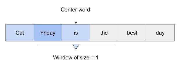
The above image shows that the context for Friday includes words like “cat” and “is”. The aim of the neural network is to predict that “Friday” falls within this context.

We activate the output layer by multiplying the vector that we passed through the hidden layer (which was the input hot vector * weights entering hidden node) with a vector representation of the context word (which is the hot vector for the context word * weights entering the output node).  The state of the output layer for the first context word can be visualised below:

The above multiplication is done for each word to context word pair. We then calculate the probability that a word belongs with a set of context words using the values resulting from the hidden and output layers. Lastly, we apply stochastic gradient descent to change the values of the weights in order to get a more desirable value for the probability calculated.

In gradient descent we need to calculate the gradient of the function being optimised at the point representing the weight that we are changing. The gradient is then used to choose the direction in which to make a step to move towards the local optimum, as shown in the minimisation example below.

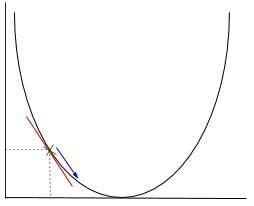
The weight will be changed by making a step in the direction of the optimal point (in the above example, the lowest point in the graph). The new value is calculated by subtracting from the current weight value the derived function at the point of the weight scaled by the learning rate.

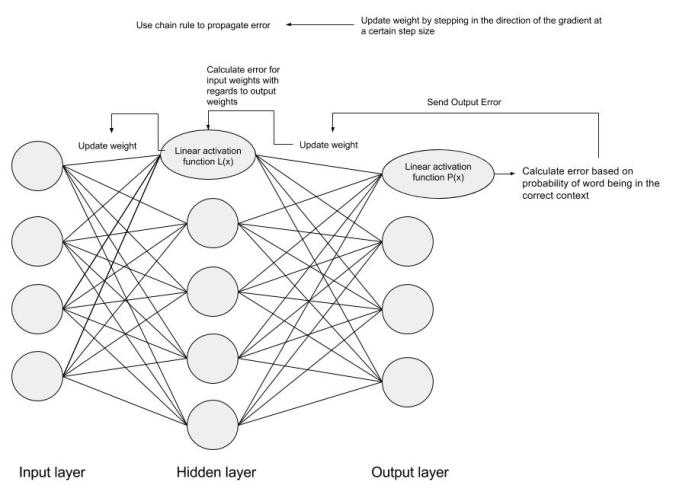
The next step is using Backpropagation, to adjust the weights between multiple layers. The error that is computed at the end of the output layer is passed back from the output layer to the hidden layer by applying the Chain Rule. Gradient descent is used to update the weights between these two layers. The error is then adjusted at each layer and sent back further. Here is a diagram to represent backpropagation:

I’m not going to go into the details of Backpropagation or gradient descent in this post. There are many great resources out there explaining the two. If you are interested in the details of these, Standford University tends to have great freely available lectures and resources on Machine learning topics.

The final vector representation of the word will be the weights (after training) that connect the input node for the word to the hidden layer. The weights connecting the hidden and output layers are representations of the context words. However, each context word is also in the vocabulary and therefore has an input representation. For this reason, the vector representation of a word is only that of the input vectors.